The playground

▶ Launch the playground — one static HTML page that runs the full rete engine in WebAssembly. No server, no account, no install: it works offline, even opened from file://. Everything below happens in your browser.

It is the fastest way to understand what rete is: pick one of the 40+ published datasets — library catalogues, citation networks, ontologies, historical maps, 3D museum collections — and query it live. The small ones are embedded in the page; the big ones (up to a 117 M-triple library graph and a 1 GB Wikidata slice) stay on their URL and are range-read lazily: a query fetches only the byte ranges it touches, and a counter shows exactly how few bytes crossed the wire.

What it looks like

Five views of the same page. Every one is a live query against a file that stays on its URL — the links reproduce each shot.

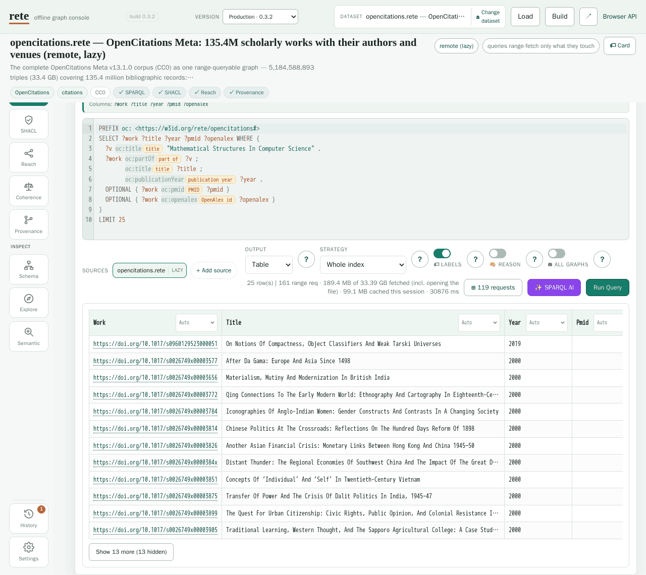
SPARQL against 5.18 billion triples. opencitations.rete is one 33.4 GB file on object storage; 25 rows cost 161 range requests and 189 MB, opening the file included. The rest is never transferred.

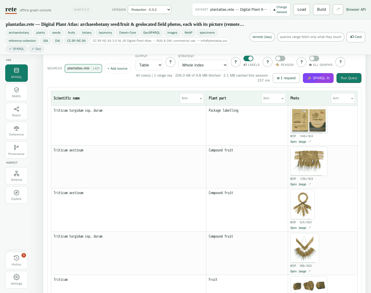
The pictures are in the graph. Those photographs are xsd:base64Binary WebP literals stored inside the .rete and rendered into the cell — 40 rows and their pictures for one range request and 256 KB. IIIF, PDF, audio, video and .glb cells work the same way; see Media & SQL companions.

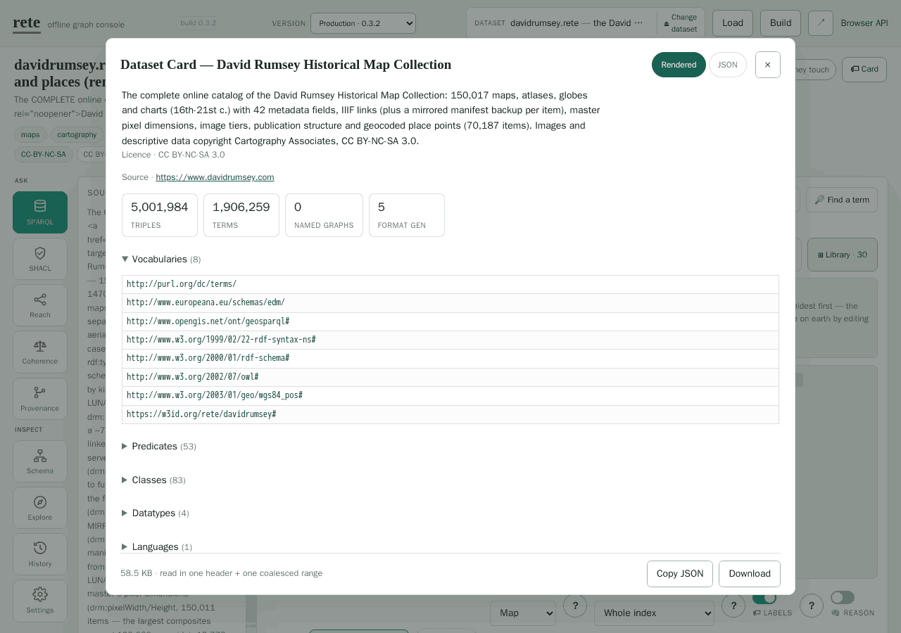
The file describes itself. The Dataset Card is read straight off the header — 58.5 KB in one coalesced range request, index untouched. See 🏷 Card below.

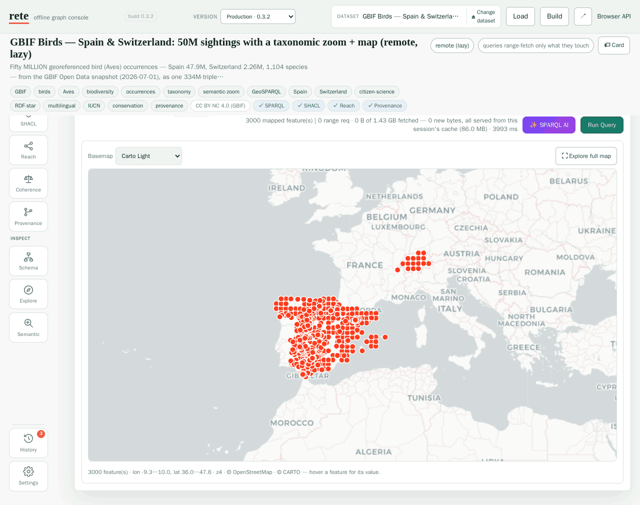
GeoSPARQL, drawn. 3,000 raptor sightings out of a 334 M-triple, 1.43 GB GBIF graph, put on a basemap — geo:asWKT detected in the result. See Output views and GeoSPARQL.

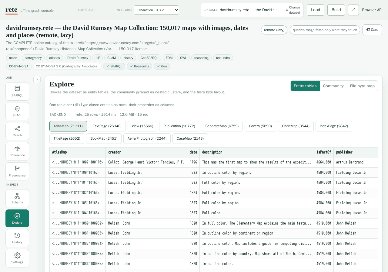
Browse it like an archive. Explore turns each rdf:type class into a table — entities as rows, properties as columns — so an unfamiliar graph is navigable before you know a predicate in it.

Pick a dataset

The dataset picker groups the catalog by theme (heritage, science, reference, demos). Each entry shows its size, license, and a description; picking one loads its example queries as one-click chips, each with a short tip explaining what the query shows. A 🔗 on every chip copies a share link that reopens the playground on that dataset with that example loaded — see Sharing a query for what that link looks like and why.

A dataset can also be sharded: one logical graph served as several files (a "⛓ N shards" chip appears). Every query fans out across the shards and the rows merge — you just query it as one dataset.

For a catalog dataset, the picker offers three load choices when applicable: Embedded uses bytes already inside the page, Lazy range-reads only what each query touches, and Cache downloads the complete .rete once. Cache mode stores the file in IndexedDB, so a reload or later browser session opens it locally with zero network reads; remove it under Settings → Whole-file caches.

Not in the catalog? + Add source → Connect (lazy) opens any .rete URL whose host serves ranges + CORS (see Hosting your .rete), and the Build mode (below) turns your own RDF into a queryable file without leaving the page.

🏷 Card — what this graph says it is

Next to the source pill, 🏷 Card opens the Dataset Card that travels inside the .rete: title, licence, source, counts, vocabularies, predicates and classes with their frequencies, the class-link skeleton, and the example queries the builder shipped with the file — plus everything the card's curated half carries: keywords and themes as tags beside the description; version, creators, publisher, DOI, canonical copy, SPARQL endpoint, source date and derived from in an Identity & provenance table; a citation with a copy button; and the publisher's own extra fields, shown last and clearly marked as theirs — rete carries those values and attaches no meaning to them.

An ORCID, ROR or DOI renders as a link to the identifier, which is why the card asks for an IRI instead of a string. A theme's IRI is not resolved (that would be a network read); the viewer names the concept scheme it can read from the IRI and shows the concept's identifier, rather than inventing a label.

Below the card, its own clearly separated part of the modal, is the build record: when the file was written, by which rete, with which flags, and what each starter query was measured to cost — those cost figures shown with the queries they describe, since that is where you ask. A file that carries no build record says so plainly instead of showing blanks.

It costs one HEAD and one header read plus one coalesced range — the card and the build record sit adjacent, so both arrive together. Never the dictionary, the index or the pyramid. That is the CARD tier: you learn what a 17 GB graph is for a few KB, before deciding whether to query it at all.

Two views: Rendered, and JSON — the card's own bytes, syntax-coloured, with Copy and Download. The JSON tab stays the card (what rete build --card-file would take); the build record lives in its own file section, outside the content hash, and is shown in the Rendered tab. Any example query the card carries has a Use button that loads it straight into the editor.

The card's queries also feed the examples panel: when a loaded file ships its own starter queries (auto-derived or curated), they appear alongside the catalog's curated examples, labelled as coming from the file's card and deduplicated against them. So a .rete you open by URL — one that was never registered in the catalog — still offers its own first questions.

Not every file has one. A card is written at build time (rete build --card …); the small bundled demo datasets are built without one, and the modal says so rather than showing an empty shell.

Write a query

The SPARQL editor comes with syntax highlighting and context autocomplete. When you don't know the graph's vocabulary yet:

🔎 Find a term browses the dataset's classes and predicates (instant, from the self-describing card) and searches entities by label — lazily over HTTP ranges on a remote graph. Click a result to drop its IRI at the cursor; each predicate offers a values › drill listing the distinct objects it takes.
Labels chips decode the IRIs in your query to human labels inline, so wd:Q937 reads as Albert Einstein while you type.
🧠 Reason (beside the Labels switch) runs the query with OWL 2 QL reasoning on — the answer then includes ontology-entailed solutions (rdfs:subClassOf / subPropertyOf / domain / range / owl:inverseOf / someValuesFrom), computed over the raw data with no materialization. So on gbif-birds, ?o a :Aves returns real occurrences via the taxonomy with the toggle on, and nothing with it off. Opt-in and lazy — over a remote dataset it fetches only what the rewritten query touches. See Reasoning by query rewriting.
⛁ All graphs (right beside 🧠 Reason) mounts the file so a pattern outside GRAPH matches the union of the default graph and every named graph — the mode Virtuoso, GraphDB and Jena TDB call the union default graph. It exists for files that keep all their data in named graphs (anything built from N-Quads), where ?s ?p ?o correctly answers zero rows; when that happens the playground points at the file's own counts and suggests the toggle. Off by default because it is not standard SPARQL; flipping it is announced, and every run under it says so in the result line. Federated runs and live endpoints keep standard semantics, and on a many-graph remote file the merge has a real byte cost — details in Union default graph.
✨ SPARQL AI drafts a query from a plain-language request using a small language model that runs locally on your GPU (WebGPU) — nothing is sent to any API. It is grounded in the dataset's example queries, so its drafts use the right vocabulary.

Results stream into the table with media-aware cells: images become thumbnails, IIIF manifests page through scans, .glb models rotate inline, WKT geometries plot on mini-maps — see Media & SQL companions for the full matrix.

Output views

The Output menu renders one result several ways. Each view expects a particular query shape — write your SELECT/CONSTRUCT so the columns it needs are present.

Output	Needs	Query shape
Table	anything	any `SELECT`, `ASK`, or `CONSTRUCT`
Cards	anything	the same rows as Table, but one card per row with the fields stacked — media renders full-width, so it reads well on a phone; on a wide screen the cards flow as a masonry. The ⚙ Fields button picks how each field renders (the same types as a table column's header dropdown).
Graph	edges to draw	a `CONSTRUCT { ?a ?p ?b } …`, or a `SELECT` with ≥ 2 variables — 2 vars are read as `v1 → v2` ("related") edges; 3 vars are read as (subject, predicate, object). A 1-variable `SELECT` has nothing to connect.
Map	a WKT geometry column	a `SELECT` that binds a variable to a `geo:wktLiteral` (e.g. `?w` via `geo:hasGeometry/geo:asWKT ?w`). `POINT` / `LINESTRING` / `POLYGON` / `MULTI` all plot; the first non-geometry* column becomes each feature's hover label.
Time	a year / date column	a `SELECT` that binds a variable to `xsd:gYear`, `xsd:date` / `xsd:dateTime`, or a plain year integer (e.g. `ex:year ?y`). The other selected column(s) become the items listed in each cell's tooltip.
TTL / JSON-LD	triples	a `CONSTRUCT` query — these serialise the constructed graph. A `SELECT` has no triples to serialise.

Rules of thumb:

Map, Time and Graph render the bindings of a SELECT, so put the geometry / year / edge columns in your SELECT list. (CONSTRUCT also feeds Graph / TTL / JSON-LD directly.)
Map and Time are available on every query (no per-dataset gating): each detects its column in the actual result and renders, or shows a short note if it's absent — so geometry or dates a query surfaces unexpectedly (e.g. from a federated join) still plot.
Run these views under the Whole index (or Split by community) strategy. Progressive answers only from the pyramid summary (counts and community structure), so it has no per-row geometry or dates to plot.
Time buckets years automatically to fit the span (per-year for short ranges, up to per-1000-year for very long ones); negative years are read as BCE. A cell's colour encodes the number of items in that bucket — hover for the list.
The map is an offline equirectangular plot of the WKT coordinates (no tiles / network), auto-fit to the bounding box of the returned geometries. A dataset that ships a PMTiles basemap adds a true tiled Output → Tiles view.

# MAP — labelled territories as polygons (history dataset)
PREFIX geo:  <http://www.opengis.net/ont/geosparql#>
PREFIX ex:   <http://ex/>
PREFIX rdfs: <http://www.w3.org/2000/01/rdf-schema#>
SELECT ?territory ?w WHERE {
  ?t ex:year 1914 ; rdfs:label ?territory ;
     geo:hasGeometry/geo:asWKT ?w .
}

# TIME — how many territories exist per year, as a multi-year heatmap
PREFIX ex:   <http://ex/>
PREFIX rdfs: <http://www.w3.org/2000/01/rdf-schema#>
SELECT ?year ?territory WHERE { ?t ex:year ?year ; rdfs:label ?territory }

# GRAPH — a 3-variable SELECT read as (subject, predicate, object)
PREFIX cito: <http://purl.org/spar/cito/>
SELECT ?a ?p ?b WHERE { ?a ?p ?b . FILTER(?p = cito:cites) } LIMIT 50

# TTL / JSON-LD — a CONSTRUCT produces serialisable triples
PREFIX cito: <http://purl.org/spar/cito/>
CONSTRUCT { ?a cito:cites ?b } WHERE { ?a cito:cites ?b } LIMIT 50

Beyond SPARQL: the other modes

The mode strip turns the same open file around several ways:

Schema — the dataset's effective schema (classes and how they relate), read index-free from the schema pyramid; the entry point for semantic zoom.
Explore — browse per-class entity tables, and (for datasets with companions) a SQL sub-tab that runs DuckDB-WASM / SQLite-WASM over the same triples as Parquet — the columnar engines and the graph engine, side by side, both lazy over HTTP.
Semantic — natural-language search over the dataset's meaning: a sentence-embedding model (running locally, multilingual) embeds your phrase and ranks entities by similarity — no keywords needed. ↗ Query these in SPARQL turns the hits into a VALUES block; ✨ Answer with AI drafts a grounded answer from them. Available on datasets that ship an embedding index.
SHACL — validate the graph against shapes in the editor; on a remote dataset only each shape's targets are range-read.
Reach — transitive reachability from seed entities along one predicate.
Provenance — "why is this triple in the result?": the physical dictionary/index/tile ranges behind a match.
Coherence — the tiered OWL coherence checks, from an index-free schema scan to full materialization (see Reasoning).
Build — paste or upload RDF (N-Triples / N-Quads / Turtle), build a real .rete in the browser, query it immediately, save it to the browser for next time, or download the file. Step 3 writes the Dataset Card the file will carry — see below. The full publish path (companions, hosting) is in Media & SQL companions and Hosting your .rete.

Writing the card in Build mode

Step 3 holds two different documents, kept apart because they are not the same thing:

the catalog entry on the left — key, icon, tags, provenance: how the dataset is listed in this playground and in a downloadable manifest. It never enters the file, and the card schema rejects those keys outright.
the Dataset Card on the right — exactly the document rete build --card-file takes, and the one that travels inside the .rete.

The JSON editor is the primary surface for the card, not a mirror of the form. It is the documented interchange format, so it cannot drift from what the CLI accepts; and the curated fields include a list of objects (creators) and a free-form bag (extra) that a form would either mangle or forbid. Title, licence, source and description also appear on the form — the four a first-time author always fills — and patch the document rather than replacing it, so typing a title never eats the creators you wrote by hand. All fields inserts a skeleton of every curated field to edit.

Validation is the engine's, not a re-statement in the page: the same code rete build --card-file runs checks what you type, with the same wording. A free-text theme is refused and pointed at keywords (where theme IRIs come from); a stray top-level key is pointed at extra; the bag's 8 KB / 64 keys / depth-2 bounds are enforced. So a card you compose here is one the CLI would also accept.

What a browser build writes, stated plainly because the difference matters to whoever reads the file later: the curated fields, and the four counts the build itself measured. It does not write the derived profile (predicates, classes, vocabularies, signals, the tiered starter-query library) or the build record. They are absent from the card rather than present-and-empty, and the 🏷 Card viewer shows that absence for what it is. Rebuild with rete build --card-file to get them (and compressed sections, which the browser cannot write).

The derived half is no longer beyond the engine's reach — the wasm build exports build_with_derived_card, which computes the whole profile in the browser from the same code the CLI runs. This page does not call it yet: derivation walks the graph twice more, and spending that on every build without asking would be the wrong default for a paste-and-see tool. The build record stays CLI-only for a different reason — its cost figures come from running the starter queries, which is a benchmark, not a build.

Leave the card editor empty and the file carries no card at all.

Federation: query several sources as one

+ Add source adds a second (third, …) .rete — from the catalog or any URL — and the query runs across all of them: union merge with predicate routing, and for flat BGPs a real cross-source join (a pattern's rows from one file joined against another's on the shared variables). See Federated queries.

A source can also be a SPARQL endpoint. With the 🔌 live checkbox the endpoint becomes the query target and SPARQL Update is enabled — pointed at a running rete serve, the playground becomes the editing UI over a live graph: INSERT DATA, watch the next SELECT reflect it, download the snapshot. (Deep-linkable as #endpoint=<url>.)

The playground keeps its entire state in the URL fragment — playground.html#dataset=<key>&load=lazy&mode=sparql&ex=<n> — so any view is reproducible from its address alone, with nothing stored server-side.

A <key> names a dataset in the catalog. To open a .rete that isn't in it — one you published yourself — give the address instead: playground.html#url=<https://…/yours.rete>&mode=sparql. It is read the same lazy way, over HTTP range requests, so the link works against a file of any size as long as its host sends Accept-Ranges: bytes and permits cross-origin reads (Access-Control-Allow-Origin, exposing Content-Range). Connecting by hand and pressing Share produces exactly this form of link.

Naming the graph and the query is not enough on its own. Several toolbar controls change what the query returns, and a link that dropped them would hand someone the same text under different semantics — the reader would see different results and have no way to tell. So the fragment also carries them, and only when they differ from the default (a plain view's link is exactly as short as it always was):

Parameter	Control	Values	Effect
`union`	⛁ All graphs	`1` / `0` (default off)	answer — mounts the file as if the default graph were the union of the default graph and every named graph
`reason`	🧠 Reason	`1` / `0` (default off)	answer — OWL 2 QL entailment, so subclass/subproperty instances also match
`strategy`	Strategy	`whole` (default) · `progressive` · `community`	answer — `progressive` answers from the pyramid summary and is approximate by contract
`round`	Round	an integer	answer — which dendrogram round the `community` strategy answers from
`fed`	SOURCES	comma-separated catalog keys, e.g. `fed=nomisma,mimotext`	answer — extra datasets the query also runs against
`view`	Output	`table` (default) · `cards` · `graph` · `map` · `tiles` · `time` · `ttl` · `jsonld`	presentation — how the same rows are drawn
`labels`	🏷 Labels	`1` (default on) / `0`	presentation — the human-label chips beside IRIs in the editor

The first five change the answer; the last two change only how it is drawn. That distinction is the design: a presentation parameter that fails to apply costs you a nicer rendering, an answer parameter that fails to apply makes the link lie. The address bar re-stamps itself as you flip these, so copying it by hand gives the same link Share does.

Federation is carried only as catalog keys. A key is a public entry in the shipped catalog, so it is short and the address is re-derived on the other side — nothing private can ride along. A source you added by pasting an address (a .rete link or a SPARQL endpoint) is deliberately left out: those are routinely intranet hosts, pre-release files, or URLs with a token in them, and a share button is not the place to forward one. When a view has such a source, Share says so instead of quietly handing out a narrower view:

Link copied ✓ — WITHOUT the added source staging: a pasted address is not put into a shareable link, so the recipient queries without it.

A fragment has one limitation: it is never sent to a server, and no link preview executes the page's JavaScript. Pasted into a chat, a feed or a search index, every deep link would therefore unfurl as the same anonymous "rete playground" card, with no hint of which graph or which question it points at.

So each catalog example and each dataset also has a small preview page of its own, and that is what 🔗 and Share copy:

Copied link	Shows
`q/<dataset>-<n>.html`	one example query: the question, the dataset, and the answer it really returns
`d/<dataset>.html`	one dataset: what it holds, how big it is, and its first example questions

Opening either one forwards you straight to the playground deep link it describes — the preview page exists for the crawler, not to slow you down. Its card is not a mock-up: every number on it was measured by actually running that query in a browser against the published file (scripts/preview/), including the range-read cost — "12 range requests · 3.5 MB of 28.7 MB read". Browse them all at Shareable queries.

An ad-hoc query has no such page (there is nothing pre-rendered to preview), so editing the SPARQL — or connecting a live endpoint, or building your own graph in the page — goes back to sharing the deep link itself, exactly as before.

So does any view carrying one of the parameters above. A preview page forwards to a link built from the catalog alone (dataset + load mode + tab + example index), which leaves it nowhere to put union=1; sharing it would silently drop exactly the setting the link exists to reproduce, so Share hands out the deep link instead.

Watching the bytes (and the caches)

For a remote dataset the result line reports what the query physically did — N range requests · M KB fetched · file is X MB — and ⊞ requests opens the actual byte-range log. Re-running a query reports "0 new bytes, all served from this session's cache" (with the cache's size — so a long, purely CPU-bound run such as a ⛁ All graphs union merge on a warm session reads as the cache working, not as a stalled fetch): reads are cached per session and — on Chromium-family browsers — fetched concurrently by default (the engine overlaps each query's byte-range requests via Asyncify, no cross-origin isolation needed; see Which browser? for why other browsers read sequentially). Settings adds further opt-in extras:

Persist fetched ranges across reloads — mirrors fetched blocks into IndexedDB (per-file usage bars + Clear), so tomorrow's session starts warm.
Whole-file caches — files downloaded through a dataset's Cache load mode survive reloads in IndexedDB and answer subsequent queries locally.
Parallel range reads — a cross-origin-isolated worker pool fetches ranges concurrently (reloads once to enable isolation; disables the CDN-loaded DuckDB/SQLite backends while on).

Which browser?

We recommend a Chromium-family browser (Chrome, Edge, Brave, …) for the playground, especially on the multi-gigabyte remote datasets. Everything works everywhere — the differences are speed and extras:

Chromium runs the concurrent reader by default: the asyncified engine fires each query's byte-range fetches in parallel, which on a big remote graph is the difference between seconds and minutes. It is the engine the playground's regression gate exercises on every change. The ✨ SPARQL AI assistant and the Semantic search tab also need WebGPU, which today means desktop Chrome/Edge.
Firefox answers every query correctly, but defaults to the reliable sequential reader: its WebAssembly engine can trap inside the concurrent reader's suspend/resume machinery once a graph is large enough (small datasets are unaffected). Sequential reads fetch the same bytes one range at a time, so large remote queries are noticeably slower. You can force concurrent reads in Settings → Concurrent reads — at the risk of the crash the default avoids.
Safari / iOS likewise defaults to sequential reads (JavaScriptCore's smaller WebAssembly stack trips the same way), and on iPhone/iPad the browser's memory ceiling can stop the very largest datasets regardless of reader.

Under the hood

The page is generated by scripts/build_playground.py from web/playground.template.html + web/playground-src/: the WASM engine, its JS glue, and the embedded datasets are inlined into one self-contained file. The JS API it drives is documented in WASM & JavaScript API; how datasets get registered is web/playground-src/catalog.js (see the repo's skills/rete-publish for the full recipe).